

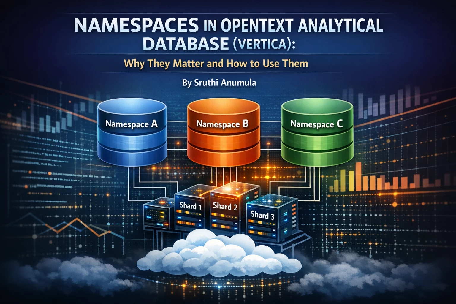


Vertica's namespace feature introduced in 24.1 represents a paradigm shift in how we architect Eon Mode databases. By enabling multiple independent shard layouts within a single database, namespaces unlock unprecedented flexibility for:
- Multi-tenant SaaS applications requiring workload isolation
- Performance optimization through right-sized shard counts per table group
- Tiered storage architectures with different access patterns
- Cost efficiency by matching infrastructure to actual needs
This guide combines theoretical understanding with practical, executable examples to help you master namespace implementation, from basic concepts to advanced architectural patterns.
The core problem namespaces solve
Before namespaces, EON mode databases had a single shard count applied universally. This created a fundamental tension: complex analytic workloads against large tables perform best when shard count matches or exceeds node count, but small tables and simple queries suffer catalog overhead from excessive shards. Organizations had to choose a compromise configuration or run separate databases.
Understanding Namespaces: Core Concepts
What Is a Namespace?
Namespaces provide the top level in Vertica's Eon Mode object hierarchy, where each namespace maintains its own shard count that defines how data is segmented across your communal storage. It sits above schemas and defines the fundamental data distribution characteristics for all objects within it. At its core, a namespace defines a global segmentation layout that all tables within it must share. Unlike Enterprise Mode where each projection could have its own segmentation scheme, Eon Mode's namespace model creates a unified hash space divided into contiguous regions, each managed by a shard. When you create a namespace with 12 shards, you're permanently defining how data flows through your cluster.
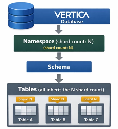
Every schema and table belongs to exactly one namespace, and every namespace has exactly one shard count that determines how data is partitioned across your cluster.
The Default Namespace
Every Eon Mode database starts with default_namespace, created automatically during database creation. If you never explicitly create additional namespaces, all your objects live here.
eonv254=> select namespace_name,is_default,default_shard_count from namespaces;
  namespace_name   | is_default | default_shard_count
-------------------+------------+---------------------
 default_namespace | t          |                   6
(1 row)
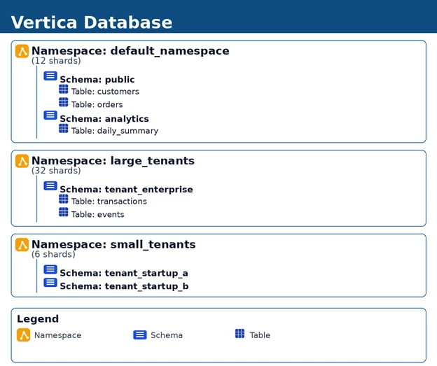
Namespace Hierarchy and Object Relationships
The picture below shows the database structure when there is more than one namespace.
Why do Namespaces Matter?
Consider three customers sharing your Vertica infrastructure. Customer A runs 500GB of data with 20 users executing predictable queries. Customer B operates at massive scale with 50TB of data, 200 users, and complex analytics workloads. Customer C needs real-time dashboards for 10 users against 5TB of data.
Customer A: 500GB data, 20 users, predictable queries
Customer B: 50TB data, 200 users, complex analytics
Customer C: 5TB data, 10 users, real-time dashboards
Without namespaces, you have three bad options:
- Single database, shared resources: Customer B's heavy queries crush everyone else's performance
- Separate Vertica clusters: 3× operational overhead, 3× licensing costs, no resource sharing
- Multiple schemas in one database: No workload isolation, shared resource pools, query interference
How Do Namespaces Solve This?
Namespaces enable flexible multi-tenant architectures by working in combination with subclusters and resource pools. When you create a namespace, you're establishing an independent execution context with its own:
- Dedicated Subclusters: Subclusters give you complete compute isolation. Customer B's heavy analytics run on their dedicated secondary subcluster while Customer C's real-time dashboards run on a separate subcluster optimized for low-latency queries.
- Independent Resource Pools: Each subcluster maintains its own resource pool hierarchy. Customer A's MEMORYSIZE, MAXCONCURRENCY, and QUEUETIMEOUT settings don't interfere with Customer B's resource allocation, even though they share the same physical cluster.
- Separate Shard Configurations: This is where performance optimization becomes powerful. You can configure different shard counts per namespace based on workload characteristics—Customer B's fact tables might use 24 shards for maximum parallelism, while Customer A's smaller datasets use 6 shards to minimize overhead and reduce metadata footprint.
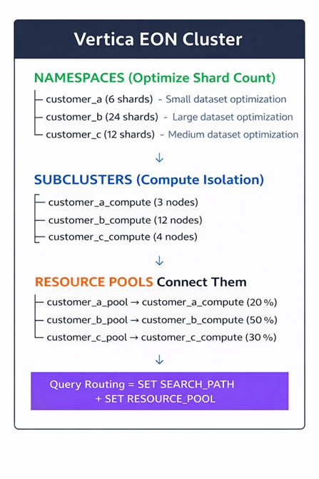
In a true multi-tenant architecture, namespaces solve the "one shard count doesn't fit all" problem by allowing different customers to have optimally sized shard counts. Combined with subclusters (compute isolation) and resource pools (memory/concurrency limits), you get enterprise-grade multi-tenancy within a single Vertica cluster.
Benefits of Namespaces
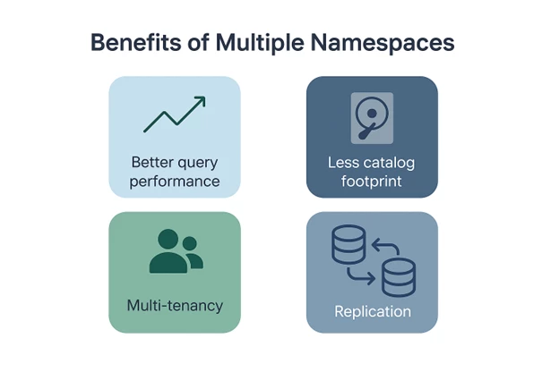
The benefits of multiple namespaces in Vertica:
- Better Query Performance: Different shard layouts for different table types (fact vs dimension, data vs text index).
- Less Catalog Footprint: Optimized shard alignment reduces metadata overhead.
- Multi-Tenancy: Enables workload isolation and faster sub-cluster spin-up.
- Replication: Supports replication across databases with different shard counts.
Shards: The Heart of Distribution
Shards are the fundamental unit of data organization in Eon Mode. Each shard isn't a physical container but rather a responsibility boundary in the hash space. Data in a namespace is divided into shards. When you create a namespace, you specify the shard count—this determines how data is partitioned across communal storage. When you insert data, Vertica hashes the segmentation key (segmentation_key_columns) to determine which shard owns that row. This hash-based distribution is deterministic and ensures even data distribution across shards.
Not all shards are created equal. Vertica uses two fundamentally different types of shards to optimize for different projection types.
1. Segment Shards (Hash-Partitioned Data)
Purpose: Distribute segmented projections (partitioned tables) across multiple shards for parallel processing.
Key Characteristics:
- Each segment shard has a hash range bound
- Data is assigned to a shard based on the hash of its segmentation key
- Only data falling within a shard's hash range will have its storage metadata (ROS containers, deletion vectors) created in that shard
- All segmented projections create and read metadata from segment shards
-- Segmented projection on a fact table
CREATE PROJECTION sales_fact_p AS
SELECT * FROM sales_fact
SEGMENTED BY HASH(customer_id) ALL NODES;
Each row is deterministically assigned to exactly one segment shard based on the hash of customer_id. The metadata for ROS files containing these rows is stored in the corresponding segment shard's metadata space.
2. Replica Shards (Unsegmented Data)
Purpose: Handle unsegmented projections (dimension tables, reference data) that need to be fully replicated across all nodes.
Key Characteristics:
- There is only ONE replica shard per namespace (no hash bounds needed)
- Contains metadata for all unsegmented projections
- All nodes automatically have access to replica shard metadata—no subscription needed
- Optimized for small, frequently joined dimension tables
-- Unsegmented projection on a dimension table
CREATE PROJECTION customer_dim_p AS
SELECT * FROM customer_dim
UNSEGMENTED ALL NODES;

-- Metadata for ALL customer_dim data stored in the single replica shard
-- Every node has a complete copy of this metadata
Design Implications: Segmented vs. Unsegmented
|
Factor |
Segmented (Segment Shards) |
Unsegmented (Replica Shard) |
|
Best For |
Large fact tables (>1GB) |
Small dimension tables (<100MB) |
|
Parallelism |
High (shard_count-way) |
Low (replicated, not parallel) |
|
Join Performance |
Requires broadcast/resegment |
Local joins, no network |
|
Storage Efficiency |
Distributed, single copy |
Replicated to all nodes |
|
Shard Pruning |
Yes (if segmentation key in WHERE) |
N/A |
|
Scaling |
Requires subscription management |
Automatic (all nodes have it) |
Understanding Default Namespace and shard subscriptions
We will be using a 25.4 EON Database having 3 nodes and running on MinIO communal Storage. Let’s verify the database details.
eonv254=> select * from namespaces;
   namespace_oid   |  namespace_name   | is_default | default_shard_count
-------------------+-------------------+------------+---------------------
 45035996273704994 | default_namespace | t          |                   6
(1 row)


eonv254=> select shard_name,shard_type,namespace_name from shards;
 shard_name  | shard_type |  namespace_name
-------------+------------+-------------------
 replica     | Replica    | default_namespace
 segment0001 | Segment    | default_namespace
 segment0002 | Segment    | default_namespace
 segment0003 | Segment    | default_namespace
 segment0004 | Segment    | default_namespace
 segment0005 | Segment    | default_namespace
 segment0006 | Segment    | default_namespace
(7 rows)
This indicates that we have one default namespace with 6 shards.
Step a: Create Sample Schema and Tables
Now let’s create segmented and unsegmented tables to understand how the data is organized.
We will create a schema named retail and a segmented table and unsegmented table.
eonv254=>CREATE SCHEMA retail;
CREATE SCHEMA

eonv254=>CREATE TABLE retail.sales_fact ( transaction_id INT, customer_id INT, product_id INT, sale_date DATE, amount DECIMAL(10,2), quantity INT );
CREATE TABLE

eonv254=>CREATE TABLE retail.product_dim ( product_id INT PRIMARY KEY, product_name VARCHAR(100), category VARCHAR(50), price DECIMAL(10,2) ) UNSEGMENTED ALL NODES;
CREATE TABLE
Step b: Load Sample Data
INSERT INTO retail.sales_fact
SELECT
    row_number() OVER () AS transaction_id,
    (random() * 1000)::INT AS customer_id,
    (random() * 100)::INT AS product_id,
    '2024-01-01'::DATE + (random() * 365)::INT AS sale_date,
    (random() * 1000)::DECIMAL(10,2) AS amount,
    (random() * 10)::INT + 1 AS quantity
FROM
    (SELECT 1 FROM v_internal.vs_nodes LIMIT 1) a,
    (SELECT 1 FROM v_internal.vs_nodes LIMIT 10000) b;

INSERT INTO retail.product_dim VALUES
    (1, 'Laptop', 'Electronics', 999.99),
    (2, 'Mouse', 'Accessories', 29.99),
    (3, 'Keyboard', 'Accessories', 79.99),
    (4, 'Monitor', 'Electronics', 299.99),
    (5, 'Desk Chair', 'Furniture', 199.99);

COMMIT;
Step c: Examine Projections and Shard Assignment
eonv254=> SELECT projection_name,projection_schema,is_segmented,segment_expression FROM projections WHERE projection_schema = 'retail';
  projection_name  | projection_schema | is_segmented |                                                              segment_expression
-------------------+-------------------+--------------+----------------------------------------------------------------------------------------------------------------------------------------------
 sales_fact_super  | retail            | t            | hash(sales_fact.transaction_id, sales_fact.customer_id, sales_fact.product_id, sales_fact.sale_date, sales_fact.amount, sales_fact.quantity)
 product_dim_super | retail            | f            |
 product_dim_super | retail            | f            |
 product_dim_super | retail            | f            |
(4 rows)

eonv254=> SELECT projection_name,shard_name,node_name FROM storage_containers WHERE schema_name = 'retail';
  projection_name  | shard_name  |     node_name
-------------------+-------------+--------------------
 product_dim_super | replica     | v_eonv254_node0001
 product_dim_super | replica     | v_eonv254_node0002
 sales_fact_super  | segment0002 | v_eonv254_node0002
 sales_fact_super  | segment0005 | v_eonv254_node0002
 product_dim_super | replica     | v_eonv254_node0003
(5 rows)
Now that we have a basic understanding of shards, Let us deep diver into shard subscription mechanics.
Shard subscription mechanics
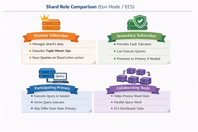
Subscriptions represent the operational contract between nodes and shards. When you add nodes to a subcluster, they start with zero subscriptions—they can't execute queries until you run REBALANCE_SHARDS (). This function redistributes shard responsibilities across available nodes, aiming for balanced distribution while maintaining K-safety
The subscription model distinguishes several node roles:
|
Role |
Description |
Responsibilities |
Key Notes |
|
Primary Subscriber |
The designated control node for a shard |
• Plans Tuple Mover operations. • Can process queries. |
• Exactly one per shard at a time |
|
Secondary Subscriber |
Standby node for high availability |
• Provides fault tolerance |
• Automatically promotes to primary on failure |
|
Participating Primary |
The node that executes a query for a shard in a session |
• Executes queries for the shard during query runtime |
• Session-dependent |
|
Collaborating Node |
Additional execution node (ECS) |
• Assists with shard data processing |
• Used in Elastic Cluster Scaling (ECS) |
The hash space division creates subtle performance characteristics that only appear on a scale. Consider what happens with a 12-shard namespace on a 12-node cluster versus a 6-shard namespace on the same cluster. In the first case, each node subscribes to exactly one shard, processing queries with perfect parallelism—when a query scans a large table, all 12 nodes work simultaneously on their respective hash space regions. In the second case, only 6 nodes participate in the query execution while the other 6 sit idle, effectively cutting your parallelism in half.
What about 6 shards with 12 nodes? Elastic Crunch Scaling (ECS), Vertica's solution to utilizing excess nodes. Let us review more about ECS in detail.
Elastic Crunch Scaling (ECS)
It is Vertica's mechanism for scaling query performance beyond shard boundaries.
Elastic Crunch Scaling (ECS) enables Vertica Eon Mode clusters to leverage compute capacity that exceeds the database's shard count, automatically splitting data processing responsibilities among multiple nodes subscribing to the same shard. When a subcluster contains more nodes than shards—for example, a 12-node subcluster in a 6-shard database—the query optimizer automatically engages ECS to ensure all nodes participate in query execution.
How ECS divides work among subscribing nodes?
The mechanism underlying ECS involves the optimizer assigning participating and collaborating node roles. In a subcluster where node count exceeds shard count, Vertica designates enough nodes as participating nodes to cover each shard (one per shard), while the remaining nodes become collaborators. Both node types process query data—the distinction relates solely to how Vertica organizes the work distribution internally.
You can identify which nodes serve which role by querying the V_CATALOG.SESSION_SUBSCRIPTIONS system table:
SELECT node_name, shard_name, is_collaborating, is_participating
FROM V_CATALOG.SESSION_SUBSCRIPTIONS
WHERE is_participating = TRUE OR is_collaborating = TRUE
ORDER BY shard_name, node_name;
In a six-node subcluster operating against a three-shard database, this query reveals three participating nodes (one per shard) and three collaborating nodes. When a query executes, Vertica assigns each node approximately half the data in its subscribed shard—effectively doubling the compute power applied to each shard's data. The optimizer indicates ECS activation in query plans with the statement "this query involves non-participating nodes," followed by a list of all nodes participating in execution.
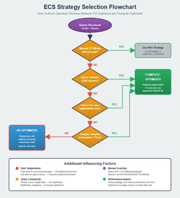
ECS Strategy Overview
The query optimizer chooses between two distinct strategies when dividing shard data among subscribing nodes, each optimized for different data access patterns and query types:
I/O-optimized strategy divides the list of ROS (Read Optimized Store) containers within each shard among subscribing nodes. Each node fetches only the specific containers assigned to it from communal storage. This strategy excels when data resides primarily in communal storage rather than the local depot, minimizing network transfer overhead. However, because container assignment is arbitrary relative to data segmentation, this approach does not preserve data segmentation and cannot support optimizations that rely on segmented data locality—queries using this strategy forfeit local join optimizations.
Compute-optimized strategy uses data segmentation to assign portions of the hash space to each subscribing node. Nodes scan the entire shard contents but apply sub-segment filtering to process only their assigned segments. This strategy is optimal when most queried data resides in the depot (local cache), since nodes must access the complete shard. The key advantage: because this strategy preserves data segmentation, it enables optimization techniques like local joins that require co-located data segments.
The optimizer automatically selects the appropriate strategy based on whether the query can benefit from data segmentation. Simple queries on single tables without joins typically receive I/O-optimized treatment, while complex queries involving JOIN or GROUP BY clauses trigger the compute-optimized strategy to preserve segmentation benefits. Query plans indicate the selection explicitly:
-- I/O-optimized (no segmentation benefit needed)
EXPLAIN SELECT employee_last_name, employee_first_name, employee_age
FROM employee_dimension ORDER BY employee_age DESC;

-- Query plan shows: "Crunch scaling strategy does not preserve data segmentation"

-- Compute-optimized (segmentation benefits JOIN)
EXPLAIN SELECT sales_quantity, sales_dollar_amount, transaction_type, cc_name
FROM online_sales.online_sales_fact
INNER JOIN online_sales.call_center_dimension
ON (online_sales_fact.call_center_key = call_center_dimension.call_center_key);

-- Query plan shows: "Crunch scaling strategy preserves data segmentation"
ECS (Elastic Crunch Scaling) currently works only on the databases with just default_namespace. Custom namespaces support standard distributed query execution with shard resegmentation, but do not support the ECS feature where non-participating nodes can dynamically assist with query processing. Full ECS support for custom namespaces is planned for future releases.
✅ How ECS Strategy Can Be Set
While automatic strategy selection handles most workloads optimally, Vertica provides multiple override mechanisms for scenarios where manual tuning improves performance.
|
Scope |
Mechanism |
Example |
Notes |
|
Database-level |
ECSMode configuration parameter |
ALTER DATABASE DEFAULT SET ECSMode='COMPUTE_OPTIMIZED'; |
Affects all sessions unless overridden |
|
Session-level |
SET SESSION ECSMode |
SET SESSION ECSMode='IO_OPTIMIZED'; |
Applies only to current session |
|
Query-level |
/*+ ECSMODE */ optimizer hint |
SELECT /*+ ECSMODE(COMPUTE_OPTIMIZED) */ ... |
Highest precedence; overrides session & database |
Now that we understand what namespaces and ECS are, let us try to understand it with simple examples.
Scenario: Query performance on namespaces with different shard count
Step 1: Verify current cluster configuration.
eonv254=> select count(*) from nodes;
 count
-------
     3
(1 row)

eonv254=> select * from namespaces;
   namespace_oid   |  namespace_name   | is_default | default_shard_count
-------------------+-------------------+------------+---------------------
 45035996273704994 | default_namespace | t          |                   6
(1 row)


eonv254=> select shard_name,shard_type,namespace_name from shards;
 shard_name  | shard_type |  namespace_name
-------------+------------+-------------------
 replica     | Replica    | default_namespace
 segment0001 | Segment    | default_namespace
 segment0002 | Segment    | default_namespace
 segment0003 | Segment    | default_namespace
 segment0004 | Segment    | default_namespace
 segment0005 | Segment    | default_namespace
 segment0006 | Segment    | default_namespace
(7 rows)
This indicates that we have 3-node cluster with default namespace with 6 shards.
Step 2: Create Namespaces with different shard count
eonv254=> CREATE NAMESPACE ecs_low SHARD COUNT 3;
CREATE NAMESPACE
eonv254=> CREATE NAMESPACE ecs_medium  SHARD COUNT 6;
CREATE NAMESPACE
eonv254=> CREATE NAMESPACE ecs_high SHARD COUNT 12;
CREATE NAMESPACE
We created 3 namespaces with different shard configurations.
Step 3: Create same table in 3 namespaces.
CREATE SCHEMA ecs_low.sales;
CREATE SCHEMA ecs_medium.sales;
CREATE SCHEMA ecs_high.sales;

-- Same table definition in all three namespaces
CREATE TABLE ecs_low.sales.transactions (
    transaction_id BIGINT,
    customer_id INT,
    product_id INT,
    store_id INT,
    transaction_date DATE,
    transaction_time TIMESTAMP,
    amount DECIMAL(10,2),
    quantity INT,
    payment_method VARCHAR(20),
    region VARCHAR(50)
);

CREATE TABLE ecs_medium.sales.transactions (
    transaction_id BIGINT,
    customer_id INT,
    product_id INT,
    store_id INT,
    transaction_date DATE,
    transaction_time TIMESTAMP,
    amount DECIMAL(10,2),
    quantity INT,
    payment_method VARCHAR(20),
    region VARCHAR(50)
);

CREATE TABLE ecs_high.sales.transactions (
    transaction_id BIGINT,
    customer_id INT,
    product_id INT,
    store_id INT,
    transaction_date DATE,
    transaction_time TIMESTAMP,
    amount DECIMAL(10,2),
    quantity INT,
    payment_method VARCHAR(20),
    region VARCHAR(50)
);
Step 4: Load the same count of rows into 3 tables.
INSERT INTO ecs_low.sales.transactions
SELECT
    row_number() OVER () as transaction_id,
    (random() * 10000)::INT + 1 as customer_id,
    (random() * 1000)::INT + 1 as product_id,
    (random() * 100)::INT + 1 as store_id,
    '2024-01-01'::DATE + (random() * 365)::INT as transaction_date,
    '2024-01-01 00:00:00'::TIMESTAMP + (random() * INTERVAL '365 days') as transaction_time,
    (10 + random() * 990)::DECIMAL(10,2) as amount,
    (random() * 10)::INT + 1 as quantity,
    CASE (random() * 4)::INT
        WHEN 0 THEN 'Credit Card'
        WHEN 1 THEN 'Debit Card'
        WHEN 2 THEN 'Cash'
        ELSE 'Mobile Pay'
    END as payment_method,
    CASE (random() * 5)::INT
        WHEN 0 THEN 'North'
        WHEN 1 THEN 'South'
        WHEN 2 THEN 'East'
        WHEN 3 THEN 'West'
        ELSE 'Central'
    END as region
FROM (
    SELECT 1
    FROM (SELECT 1 UNION ALL SELECT 1 UNION ALL SELECT 1 UNION ALL SELECT 1 UNION ALL
          SELECT 1 UNION ALL SELECT 1 UNION ALL SELECT 1 UNION ALL SELECT 1 UNION ALL
          SELECT 1 UNION ALL SELECT 1) t1  -- 10 rows
    CROSS JOIN (SELECT 1 UNION ALL SELECT 1 UNION ALL SELECT 1 UNION ALL SELECT 1 UNION ALL
                SELECT 1 UNION ALL SELECT 1 UNION ALL SELECT 1 UNION ALL SELECT 1 UNION ALL
                SELECT 1 UNION ALL SELECT 1) t2  -- 10 rows = 100 total
    CROSS JOIN (SELECT 1 UNION ALL SELECT 1 UNION ALL SELECT 1 UNION ALL SELECT 1 UNION ALL
                SELECT 1 UNION ALL SELECT 1 UNION ALL SELECT 1 UNION ALL SELECT 1 UNION ALL
                SELECT 1 UNION ALL SELECT 1) t3  -- 10 rows = 1,000 total
    CROSS JOIN (SELECT 1 UNION ALL SELECT 1 UNION ALL SELECT 1 UNION ALL SELECT 1 UNION ALL
                SELECT 1 UNION ALL SELECT 1 UNION ALL SELECT 1 UNION ALL SELECT 1 UNION ALL
                SELECT 1 UNION ALL SELECT 1) t4  -- 10 rows = 10,000 total
    CROSS JOIN (SELECT 1 UNION ALL SELECT 1 UNION ALL SELECT 1 UNION ALL SELECT 1 UNION ALL
                SELECT 1 UNION ALL SELECT 1 UNION ALL SELECT 1 UNION ALL SELECT 1 UNION ALL
                SELECT 1 UNION ALL SELECT 1) t5  -- 10 rows = 100,000 total
) x;
OUTPUT
--------
 100000
(1 row)

eonv254=>  INSERT INTO ecs_medium.sales.transactions select * from ecs_low.sales.transactions;
 OUTPUT
--------
 100000
(1 row)

eonv254=>  INSERT INTO ecs_high.sales.transactions select * from ecs_low.sales.transactions;
 OUTPUT
--------
 100000
(1 row)

eonv254=>
Step 5: Let us run a simple aggregation query against the 3 tables
eonv254=> \timing on
Timing is on.
eonv254=> SELECT
eonv254->     transaction_date,
eonv254->     region,
eonv254->     payment_method,
eonv254->     COUNT(*) as txn_count,
eonv254->     ROUND(SUM(amount)::NUMERIC, 2) as daily_sales
eonv254-> FROM ecs_low.sales.transactions
eonv254-> WHERE transaction_date >= '2024-06-01'
eonv254-> GROUP BY transaction_date, region, payment_method
eonv254-> ORDER BY transaction_date DESC, daily_sales DESC
eonv254-> LIMIT 10;
 transaction_date | region  | payment_method | txn_count | daily_sales
------------------+---------+----------------+-----------+-------------
 2024-12-31       | Central | Mobile Pay     |        21 |     9458.84
 2024-12-31       | East    | Mobile Pay     |        16 |     9388.09
 2024-12-31       | Central | Cash           |        15 |     6852.61
 2024-12-31       | Central | Debit Card     |        12 |     6682.10
 2024-12-31       | South   | Mobile Pay     |         8 |     3795.62
 2024-12-31       | South   | Debit Card     |         6 |     3354.27
 2024-12-31       | North   | Mobile Pay     |         5 |     3187.85
 2024-12-31       | East    | Cash           |         6 |     3102.80
 2024-12-31       | East    | Credit Card    |         6 |     2989.51
 2024-12-31       | Central | Credit Card    |         5 |     2638.36
(10 rows)

Time: First fetch (10 rows): 96.321 ms. All rows formatted: 96.609 ms
eonv254=> SELECT
eonv254->     transaction_date,
eonv254->     region,
eonv254->     payment_method,
eonv254->     COUNT(*) as txn_count,
eonv254->     ROUND(SUM(amount)::NUMERIC, 2) as daily_sales
eonv254-> FROM ecs_medium.sales.transactions
eonv254-> WHERE transaction_date >= '2024-06-01'
eonv254-> GROUP BY transaction_date, region, payment_method
eonv254-> ORDER BY transaction_date DESC, daily_sales DESC
eonv254-> LIMIT 10;
 transaction_date | region  | payment_method | txn_count | daily_sales
------------------+---------+----------------+-----------+-------------
 2024-12-31       | Central | Mobile Pay     |        21 |     9458.84
 2024-12-31       | East    | Mobile Pay     |        16 |     9388.09
 2024-12-31       | Central | Cash           |        15 |     6852.61
 2024-12-31       | Central | Debit Card     |        12 |     6682.10
 2024-12-31       | South   | Mobile Pay     |         8 |     3795.62
 2024-12-31       | South   | Debit Card     |         6 |     3354.27
 2024-12-31       | North   | Mobile Pay     |         5 |     3187.85
 2024-12-31       | East    | Cash           |         6 |     3102.80
 2024-12-31       | East    | Credit Card    |         6 |     2989.51
 2024-12-31       | Central | Credit Card    |         5 |     2638.36
(10 rows)

Time: First fetch (10 rows): 93.295 ms. All rows formatted: 93.413 ms
eonv254=> SELECT
eonv254->     transaction_date,
eonv254->     region,
eonv254->     payment_method,
eonv254->     COUNT(*) as txn_count,
eonv254->     ROUND(SUM(amount)::NUMERIC, 2) as daily_sales
eonv254-> FROM ecs_high.sales.transactions
eonv254-> WHERE transaction_date >= '2024-06-01'
eonv254-> GROUP BY transaction_date, region, payment_method
eonv254-> ORDER BY transaction_date DESC, daily_sales DESC
eonv254-> LIMIT 10;
 transaction_date | region  | payment_method | txn_count | daily_sales
------------------+---------+----------------+-----------+-------------
 2024-12-31       | Central | Mobile Pay     |        21 |     9458.84
 2024-12-31       | East    | Mobile Pay     |        16 |     9388.09
 2024-12-31       | Central | Cash           |        15 |     6852.61
 2024-12-31       | Central | Debit Card     |        12 |     6682.10
 2024-12-31       | South   | Mobile Pay     |         8 |     3795.62
 2024-12-31       | South   | Debit Card     |         6 |     3354.27
 2024-12-31       | North   | Mobile Pay     |         5 |     3187.85
 2024-12-31       | East    | Cash           |         6 |     3102.80
 2024-12-31       | East    | Credit Card    |         6 |     2989.51
 2024-12-31       | Central | Credit Card    |         5 |     2638.36
(10 rows)

Time: First fetch (10 rows): 100.745 ms. All rows formatted: 101.043 ms
Based on the above results, we notice that query is performing faster in a namespace with 6 shards.
|
Namespace |
Shards |
Ratio |
Time (ms) |
Performance |
|
ecs_low |
3 |
1:1 |
96.3 |
Slower (limited parallelism) |
|
ecs_medium |
6 |
2:1 |
93.3 |
FASTEST ✓ |
|
ecs_high |
12 |
4:1 |
100.7 |
Slowest (overhead > benefit) |
Why ecs_medium Won:
✅ Sweet spot for this workload - Enough parallelism (6-way) to distribute work efficiently
✅ Balanced overhead - Not too much coordination cost like high shard count
✅ Optimal for moderate queries - This query doesn't benefit from 12-way parallelism
Key Insight:
More shards ≠ always faster!
The 6-shard (2:1 ratio) configuration provides the best balance between parallelism and coordination overhead. Choose shard count based on your actual query patterns, not just "more is better."
Scenario: Query performance with and without ECS Strategy
Step 1: Currently ECS works only on databases without custom namespaces. Drop all the tables and then namespaces.
eonv254=> drop schema ecs_single.sales cascade;
DROP SCHEMA
eonv254=> drop schema ecs_low.sales cascade;
DROP SCHEMA
eonv254=> drop schema ecs_high.sales cascade;
DROP SCHEMA
eonv254=> drop schema ecs_medium.sales cascade;
DROP SCHEMA
eonv254=> DROP NAMESPACE IF EXISTS ecs_single;
DROP NAMESPACE
eonv254=> DROP NAMESPACE IF EXISTS ecs_medium;
DROP NAMESPACE
eonv254=> DROP NAMESPACE IF EXISTS ecs_low;
DROP NAMESPACE
eonv254=> DROP NAMESPACE IF EXISTS ecs_high;
DROP NAMESPACE
eonv254=> select * from namespaces;
   namespace_oid   |  namespace_name   | is_default | default_shard_count
-------------------+-------------------+------------+---------------------
 45035996273704994 | default_namespace | t          |                   6
(1 row)
Step 2: Reshard the database.
Execute RESHARD_DATABASE(1) to reduce the default_namespace shard count from 6 to 1. This intentionally creates an imbalanced configuration where nodes outnumber shards (3:1 ratio), enabling the 'non-participating nodes' ECS scenario. Production systems should maintain shard counts near or equal to node counts for proper distribution.
eonv254=>     select reshard_database(1);
WARNING 10680:  The new shard count is not optimal one
HINT:  Please set the shard count to a multiple of 12 to maximize the combination of subcluster topologies
             reshard_database
------------------------------------------
 Database re-sharding has been completed.
(1 row)

eonv254=> select rebalance_shards();
 rebalance_shards
-------------------
 REBALANCED SHARDS
(1 row)
Step 3: create a table and load data
CREATE TABLE public.sales_transactions (
    transaction_id BIGINT,
    customer_id INT,
    product_id INT,
    store_id INT,
    transaction_date DATE,
    transaction_time TIMESTAMP,
    amount DECIMAL(10,2),
    quantity INT,
    payment_method VARCHAR(20),
    region VARCHAR(50)
) ORDER BY transaction_date, customer_id
SEGMENTED BY HASH(customer_id) ALL NODES;
INSERT INTO public.sales_transactions
SELECT
    row_number() OVER () as transaction_id,
    (random() * 10000)::INT + 1 as customer_id,
    (random() * 1000)::INT + 1 as product_id,
    (random() * 100)::INT + 1 as store_id,
    '2024-01-01'::DATE + (random() * 365)::INT as transaction_date,
    '2024-01-01 00:00:00'::TIMESTAMP + (random() * INTERVAL '365 days') as transaction_time,
    (10 + random() * 990)::DECIMAL(10,2) as amount,
    (random() * 10)::INT + 1 as quantity,
    CASE (random() * 4)::INT
        WHEN 0 THEN 'Credit Card'
        WHEN 1 THEN 'Debit Card'
        WHEN 2 THEN 'Cash'
        ELSE 'Mobile Pay'
    END as payment_method,
    CASE (random() * 5)::INT
        WHEN 0 THEN 'North'
        WHEN 1 THEN 'South'
        WHEN 2 THEN 'East'
        WHEN 3 THEN 'West'
        ELSE 'Central'
    END as region
FROM (
    SELECT 1
    FROM (SELECT 1 UNION ALL SELECT 1 UNION ALL SELECT 1 UNION ALL SELECT 1 UNION ALL
          SELECT 1 UNION ALL SELECT 1 UNION ALL SELECT 1 UNION ALL SELECT 1 UNION ALL
          SELECT 1 UNION ALL SELECT 1) t1
    CROSS JOIN (SELECT 1 UNION ALL SELECT 1 UNION ALL SELECT 1 UNION ALL SELECT 1 UNION ALL
                SELECT 1 UNION ALL SELECT 1 UNION ALL SELECT 1 UNION ALL SELECT 1 UNION ALL
                SELECT 1 UNION ALL SELECT 1) t2
    CROSS JOIN (SELECT 1 UNION ALL SELECT 1 UNION ALL SELECT 1 UNION ALL SELECT 1 UNION ALL
                SELECT 1 UNION ALL SELECT 1 UNION ALL SELECT 1 UNION ALL SELECT 1 UNION ALL
                SELECT 1 UNION ALL SELECT 1) t3
    CROSS JOIN (SELECT 1 UNION ALL SELECT 1 UNION ALL SELECT 1 UNION ALL SELECT 1 UNION ALL
                SELECT 1 UNION ALL SELECT 1 UNION ALL SELECT 1 UNION ALL SELECT 1 UNION ALL
                SELECT 1 UNION ALL SELECT 1) t4
    CROSS JOIN (SELECT 1 UNION ALL SELECT 1 UNION ALL SELECT 1 UNION ALL SELECT 1 UNION ALL
                SELECT 1 UNION ALL SELECT 1 UNION ALL SELECT 1 UNION ALL SELECT 1 UNION ALL
                SELECT 1 UNION ALL SELECT 1) t5
    CROSS JOIN (SELECT 1 UNION ALL SELECT 1 UNION ALL SELECT 1 UNION ALL SELECT 1 UNION ALL
                SELECT 1) t6  -- 10 × 10 × 10 × 10 × 10 × 5 = 500,000
) x;

COMMIT;
Step 4: Run explain plan of the query
We notice "non-participating nodes" message in EXPLAIN output which indicates that ECS Strategy has kicked in.
explain SELECT
     region,
     payment_method,
     COUNT(*) as total_transactions,
     COUNT(DISTINCT customer_id) as unique_customers,
     COUNT(DISTINCT product_id) as unique_products,
     SUM(amount) as total_revenue,
     AVG(amount) as avg_transaction
 FROM public.sales_transactions
 GROUP BY region, payment_method
 ORDER BY total_revenue DESC;

                                                                                                                                                                                      QUERY PLAN


----------------------------------------------------------------------------------------------------------------------------------------------------------------------------------------------------------
----------------------------------------------------------------------------------------------------------------------------------------------------------------------------------------------------------
----------------------------------------------------------------------------------------------------------------------------------------------------------------------------------------------------------
----------------------------------------------------------------------------------------------------------------------------------------------------------------------------
 ------------------------------
 QUERY PLAN DESCRIPTION:
 The execution of this query involves non-participating nodes. Crunch scaling strategy preserves data segmentation
 ------------------------------

 EE Vertica Options
 --------------------
 ENABLE_JOIN_SPILL


 explain SELECT
      region,
      payment_method,
      COUNT(*) as total_transactions,
      COUNT(DISTINCT customer_id) as unique_customers,
      COUNT(DISTINCT product_id) as unique_products,
      SUM(amount) as total_revenue,
      AVG(amount) as avg_transaction
  FROM public.sales_transactions
  GROUP BY region, payment_method
  ORDER BY total_revenue DESC;

 Access Path:
 +-SORT [Cost: 16K, Rows: 10K] (PATH ID: 1)
 |  Order: "Sqry$_1".total_revenue DESC
 |  Execute on: All Nodes
 | +---> JOIN MERGEJOIN(inputs presorted) [Cost: 15K, Rows: 10K] (PATH ID: 2)
 | |      Join Cond: ("Sqry$_1".region <=> "Sqry$_2".region) AND ("Sqry$_1".payment_method <=> "Sqry$_2".payment_method)
 | |      Execute on: All Nodes
 | | +-- Outer -> SELECT [Cost: 3K, Rows: 10K] (PATH ID: 3)
 | | |      Execute on: All Nodes
 | | | +---> GROUPBY HASH (SORT OUTPUT) (GLOBAL RESEGMENT GROUPS) (LOCAL RESEGMENT GROUPS) [Cost: 3K, Rows: 10K] (PATH ID: 4)
 | | | |      Aggregates: count(DISTINCT sales_transactions.customer_id), sum_of_count(*), sum(<SVAR>), sum_float(<SVAR>), sum_of_count(<SVAR>)
 | | | |      Group By: sales_transactions.region, sales_transactions.payment_method
 | | | |      Execute on: All Nodes
 | | | |      Runtime Filters: (SIP1(MergeJoin): "Sqry$_1".region), (SIP2(MergeJoin): "Sqry$_1".payment_method), (SIP3(MergeJoin): "Sqry$_1".region, "Sqry$_1".payment_method)
 | | | | +---> GROUPBY HASH (LOCAL RESEGMENT GROUPS) [Cost: 2K, Rows: 10K] (PATH ID: 5)
 | | | | |      Aggregates: count(*), sum(sales_transactions.amount), sum_float(sales_transactions.amount), count(sales_transactions.amount)
 | | | | |      Group By: sales_transactions.region, sales_transactions.payment_method, sales_transactions.customer_id
 | | | | |      Execute on: All Nodes
 | | | | | +---> STORAGE ACCESS for sales_transactions [Cost: 2K, Rows: 500K] (PATH ID: 6)
 | | | | | |      Projection: default_namespace.public.sales_transactions_super
 | | | | | |      Materialize: sales_transactions.customer_id, sales_transactions.amount, sales_transactions.payment_method, sales_transactions.region
 | | | | | |      Execute on: All Nodes
 | | +-- Inner -> SELECT [Cost: 12K, Rows: 1K] (PATH ID: 7)
 | | |      Execute on: All Nodes
 | | | +---> GROUPBY HASH (SORT OUTPUT) (GLOBAL RESEGMENT GROUPS) (LOCAL RESEGMENT GROUPS) [Cost: 12K, Rows: 1K] (PATH ID: 8)
 | | | |      Aggregates: count(DISTINCT sales_transactions.product_id)
 | | | |      Group By: sales_transactions.region, sales_transactions.payment_method
 | | | |      Execute on: All Nodes
 | | | | +---> GROUPBY HASH (GLOBAL RESEGMENT GROUPS) (LOCAL RESEGMENT GROUPS) [Cost: 12K, Rows: 1K] (PATH ID: 9)
 | | | | |      Group By: sales_transactions.region, sales_transactions.payment_method, sales_transactions.product_id
 | | | | |      Execute on: All Nodes
 | | | | | +---> STORAGE ACCESS for sales_transactions [Cost: 1K, Rows: 500K] (PATH ID: 10)
 | | | | | |      Projection: default_namespace.public.sales_transactions_super
 | | | | | |      Materialize: sales_transactions.product_id, sales_transactions.payment_method, sales_transactions.region
 | | | | | |      Execute on: All Nodes
Step 5: Verify collaborating nodes using session subscriptions.
The output shows the following ECS behavior:
- Node 1 (participating): Scans data from Shard 1
- Nodes 2 & 3 (non-participating): Receive redistributed data and assist with aggregation
- Result: All 3 nodes collaborate on processing, even though only 1 node has data
eonv253=> select node_name,shard_name,is_participating,is_collaborating from session_subscriptions order by node_name;
     node_name      | shard_name  | is_participating | is_collaborating
--------------------+-------------+------------------+------------------
 v_eonv253_node0001 | replica     | t                | f
 v_eonv253_node0001 | segment0001 | t                | f
 v_eonv253_node0002 | replica     | f                | t
 v_eonv253_node0002 | segment0001 | f                | t
 v_eonv253_node0003 | replica     | f                | t
 v_eonv253_node0003 | segment0001 | f                | t
Step 6: Run sample query with and without ECS Strategy.
SELECT /*+ECSMode(NONE)*/
    t1.region,
    t1.payment_method,
    COUNT(DISTINCT t1.customer_id) as unique_customers,
    COUNT(DISTINCT t2.product_id) as unique_products,
    SUM(t1.amount * t2.amount) as cross_product_sum,
    AVG(t1.amount * t2.amount) as cross_product_avg
FROM public.sales_transactions t1
CROSS JOIN public.sales_transactions t2
WHERE t1.customer_id = t2.customer_id
  AND t1.transaction_date >= '2024-06-01'
  AND t2.transaction_date >= '2024-06-01'
GROUP BY t1.region, t1.payment_method;
SELECT /*+ECSMode(COMPUTE_OPTIMIZED)*/
    t1.region,
    t1.payment_method,
    COUNT(DISTINCT t1.customer_id) as unique_customers,
    COUNT(DISTINCT t2.product_id) as unique_products,
    SUM(t1.amount * t2.amount) as cross_product_sum,
    AVG(t1.amount * t2.amount) as cross_product_avg
FROM public.sales_transactions t1
CROSS JOIN public.sales_transactions t2
WHERE t1.customer_id = t2.customer_id
  AND t1.transaction_date >= '2024-06-01'
  AND t2.transaction_date >= '2024-06-01'
GROUP BY t1.region, t1.payment_method;
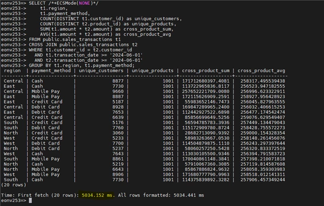
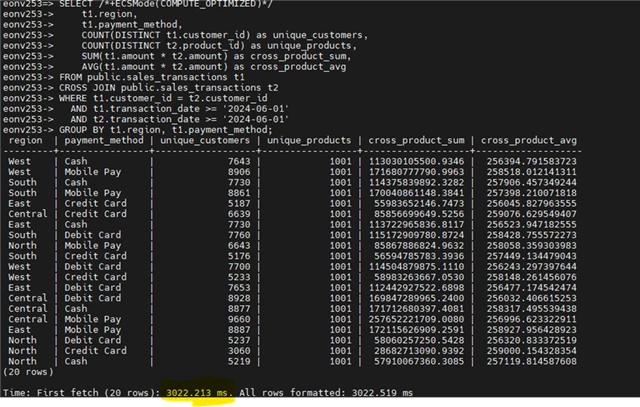
📊 Query Performance Results:
|
ECS Mode |
Execution Time |
Performance vs NONE |
|
COMPUTE_OPTIMIZED |
3,022 ms |
🚀 40% FASTER |
|
NONE (disabled) |
5,034 ms |
Baseline |
Elastic Crunch Scaling (ECS) demonstrated a 40% performance improvement (5,034ms → 3,022ms) on a compute-intensive self-join query with multiple DISTINCT aggregations. By distributing the computational workload across all 3 nodes—including 2 non-participating nodes with no shard subscriptions—ECS effectively leveraged idle compute resources to accelerate query execution. This proves that ECS provides measurable benefits for complex analytical queries where compute operations dominate over I/O, making it valuable for workloads involving joins, multiple aggregations, and heavy calculations.
ECS is not a universal speedup, it’s targeted optimization for compute and I/O bound queries
This deep dive into Vertica namespaces and ECS revealed critical insights about distributed query optimization. The demonstrations and scripts shared here provide a foundation for your own testing. Adapt them to your data volumes, query patterns, and infrastructure constraints.
Test. Measure. Optimize. Repeat.
The best Vertica architecture is the one that fits YOUR data. 📊
Additional Information
Manually choosing an ECS strategy